用mle分段拟合损失分布,并计算模拟随机数
-
因为保险损失程度分布是long tail的,所以需要有时需要对不同段的损失拟合不同分布。
这里的思路是先分段,假设好损失出现在每段的概率,然后对每段数据进行分别拟合。
分别拟合会遇到Density的积分加起来不等于1的情况,因此,还需要对每段的Density函数用一个系数进行调整,来达到把总和调整为1的效果。
-
样本代码如下,假设分三段 [0-50], [50-120], [120-250]; 每段的概率是0.2, 0.5, 0.3;
FitThreeDBs这个函数会在每个模型跑出来的参数里面加一个系数,这个系数要×在Density Function上,来实现把Density总和调整到1的效果。
# 四个参数,数据,分段点,拟合的分布名,以及每段的概率
FitThreeDBs = function(data,breaks,fittedDBs,probabilities){
#把拟合数据分段
  data2cut<-
    cut(data, breaks = breaks,
        include.lowest = TRUE)
#储存每段的模型
  model = list()
  for(i in 1:(length(breaks)-1)){
    if(length(data)<2){
#如果某段数据量小于2,那么不输出模型
      model= c(model,"")
    print("warning")
    }
    else{
#拟合这段数据的模型
      temp_model = fitdistr(unlist(split(data,data2cut)[i]), fittedDBs[i])

    }
#计算调整系数,调整系数应该等于在拟合数据范围我们想要的概率,除以拟合出的分布在拟合数据范围的概率
    point1 = do.call(paste0("p",fittedDBs[i]), list(breaks[i+1],temp_model$estimate[1],temp_model\$estimate[2]))
    point2 =  do.call(paste0("p",fittedDBs[i]), list(breaks[i],temp_model$estimate[1],temp_model\$estimate[2]))
    temp_model["coefficient"] <- probabilities[i]/(point1-point2)
    model[[length(model)+1]]= temp_model
  }
  return(model)
}

#Simulation data是拟合数据
modelCollections = FitThreeDBs(simulation_data,c(0,50,120,250),c("gamma","weibull","gamma"),c(0.2,0.5,0.3))
-
验证了一下,总和确实为1
sum = pgamma(50,shape=modelCollections[[1]]\$estimate["shape"], rate=modelCollections[[1]]\$estimate["rate"])*modelCollections[[1]]['coefficient'][[1]]
sum = sum + (pweibull(120,modelCollections[[2]]\$estimate["shape"],modelCollections[[2]]\$estimate["scale"])-
                      pweibull(50,modelCollections[[2]]\$estimate["shape"]
                               ,modelCollections[[2]]\$estimate["scale"]))*modelCollections[[2]]['coefficient'][[1]]
sum = sum + (pgamma(250,modelCollections[[3]]$estimate["shape"]
                    ,modelCollections[[3]]\$estimate["rate"])- pgamma(120,modelCollections[[3]]\$estimate["shape"]
                                                                     ,modelCollections[[3]]\$estimate["rate"]))*modelCollections[[3]]['coefficient'][[1]]

#输出Sum,结果为1
-
那么,如何用拟合出来的分布做Simulation呢,就要用到一个知识点,那就是可以先生成服从0到1之间均匀分布的随机数,再Map到拟合分段函数的CDF $F(x)$上,然后计算该概率下的quantile就是最后的随机数。
分段函数的CDF $F(x)$是由每段函数原本的CDF通过改变截距和形状来的,那么我们就可以把它还原到原来函数的CDF,用R的功能计算出quantile来
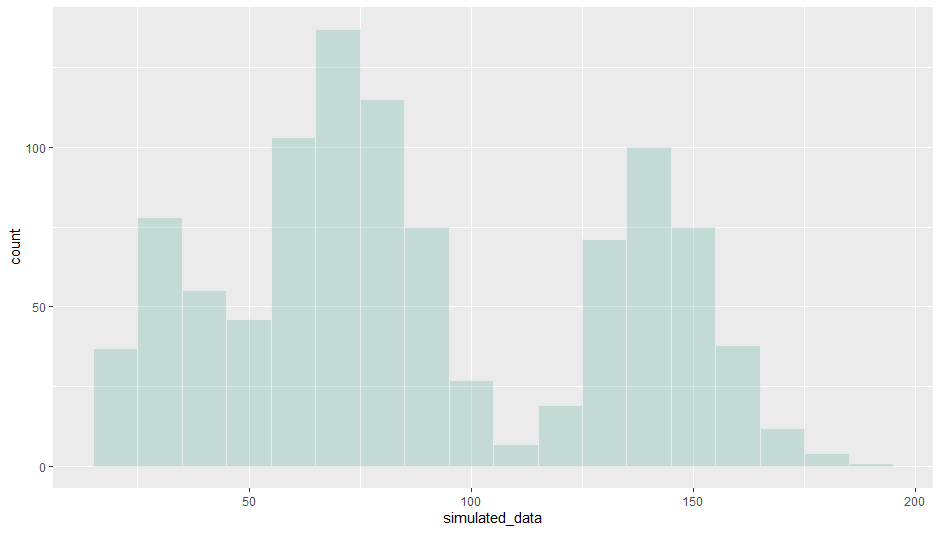
#生成1000个符合0-1之间均匀分布的随机数
init_numebrs = runif(1000)

simulation = function(init){
#这两个break就是CDF的分段点
  break1=  0.2
  break2 = 0.2+0.5
 #这里就是把改变形状截距的CDF还原回去,然后计算quantile
  if(init<break1){
    output = qgamma(init/modelCollections[[1]]['coefficient'][[1]],shape=modelCollections[[1]]\$estimate["shape"], rate=modelCollections[[1]]\$estimate["rate"])
  }else if(init>break2){
    output = qgamma((init-break2)/modelCollections[[3]]['coefficient'][[1]]+pgamma(120,modelCollections[[3]]\$estimate["shape"],modelCollections[[3]]\$estimate["rate"]),shape=modelCollections[[3]]\$estimate["shape"], rate=modelCollections[[3]]\$estimate["rate"])
  }else{
    output = qweibull((init-break1)/modelCollections[[2]]['coefficient'][[1]]+pweibull(50,modelCollections[[2]]\$estimate["shape"],modelCollections[[2]]\$estimate["scale"]),shape=modelCollections[[2]]\$estimate["shape"], scale=modelCollections[[2]]\$estimate["scale"])

  }
}

simulation_result=lapply(init_numebrs,simulation)

dt = data.frame("data"=unlist(simulation_result))
p = ggplot(data = data.frame(dt), aes(x = data)) + geom_histogram(binwidth=10,fill="#69b3a2", color="#e9ecef", alpha=0.3)
拟合出来的分布大概是以下形状